8.5 Medoids
import numpy as np
import matplotlib.pyplot as plt
from scipy.stats import multivariate_normal

mu = [0, 0]
sig = [1, 1]
rho = -0.3

cov = rho * np.sqrt(sig[0] * sig[1])
sigma = [[sig[0], cov], [cov, sig[1]]]

N = 10

points = multivariate_normal.rvs(mean=mu, cov=sigma, size=N)
points = np.sort(points, axis=0)

mn, mx = np.floor(points.min()), np.ceil(points.max())

distances = np.zeros((N, 3))
for i in range(N):
    dv = points - points[i]
    d = np.sum(dv**2, axis=1)
    d1 = np.sqrt(d)
    d2 = np.sum(np.abs(dv), axis=1)
    distances[i, 0] = np.sum(d)
    distances[i, 1] = np.sum(d1)
    distances[i, 2] = np.sum(d2)

dmu = points[np.argmin(distances[:, 0])]
dmu1 = points[np.argmin(distances[:, 1])]
dmu2 = points[np.argmin(distances[:, 2])]

emu = np.mean(points, axis=0)

emu1, emu2 = emu.copy(), emu.copy()
for _ in range(100):
    dv1 = points - emu1
    dv2 = points - emu2
    d1 = np.linalg.norm(dv1, axis=1)
    d2 = np.sum(np.abs(dv2), axis=1)
    emu1 = np.sum(points / d1[:, None], axis=0) / np.sum(1 / d1)
    emu2 = np.sum(points / d2[:, None], axis=0) / np.sum(1 / d2)

plt.figure()
plt.scatter(points[:, 0], points[:, 1], marker='+', color='k', label='Data Points')
plt.scatter(*emu, color='r', marker='o', label='Mean')
plt.scatter(*emu1, color='b', marker='o', label='Geometric Median')
plt.scatter(*dmu, color='r', marker='s', label='Squared Euclidean Medoid')
plt.scatter(*dmu1, color='b', marker='s', label='Euclidean Medoid')
plt.scatter(*dmu2, color='g', marker='s', label='Manhattan Medoid')
plt.legend(loc='lower left')
plt.xlim(mn, mx)
plt.ylim(mn, mx)
plt.gca().set_aspect('equal', adjustable='box')
plt.grid()
plt.show()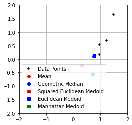
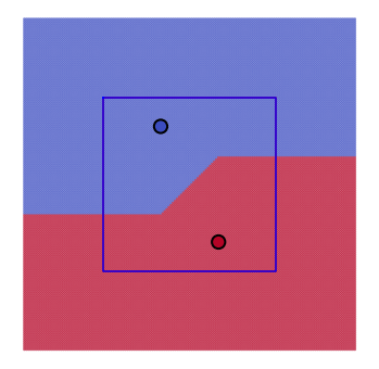
8.6 Roc Callin
import numpy as np
import matplotlib.pyplot as plt
from scipy.stats import multivariate_normal
from sklearn.neighbors import KNeighborsClassifier

Tr = np.array([[-7, 14], [7, -14]])
Cl = np.array([1, 2])

Nexemplars = Tr.shape[0]
mn, mx = -40, 40
N = 2 * (mx - mn)

Te = np.array([[mn + j * (mx - mn) / N, mn + i * (mx - mn) / N]
                for i in range(N + 1) for j in range(N + 1)])

methods = ['euclidean', 'manhattan']
for m, method in enumerate(methods):
    for k in range(1, Nexemplars):
        plt.figure(figsize=(6, 6))
        plt.axis([mn, mx, mn, mx])
        plt.axis('equal')
        plt.axis('off')

        knn = KNeighborsClassifier(n_neighbors=k, metric=method)
        knn.fit(Tr, Cl)
        Lb = knn.predict(Te)

        plt.scatter(Te[:, 0], Te[:, 1], c=Lb, s=3, cmap='coolwarm', alpha=0.5)
        plt.scatter(Tr[:, 0], Tr[:, 1], c=Cl, s=150, edgecolors='k', linewidth=2, cmap='coolwarm')

        if k == 1 and method == 'euclidean':
            circle = plt.Circle((0, 0), np.linalg.norm(Tr[0]), color='m', fill=False)
            plt.gca().add_patch(circle)
        elif k == 1 and method == 'manhattan':
            plt.plot([-21, 21, 21, -21, -21], [21, 21, -21, -21, 21], 'r')
            plt.plot([-21, 21, 21, -21, -21], [21, 21, -21, -21, 21], 'b')

        plt.show()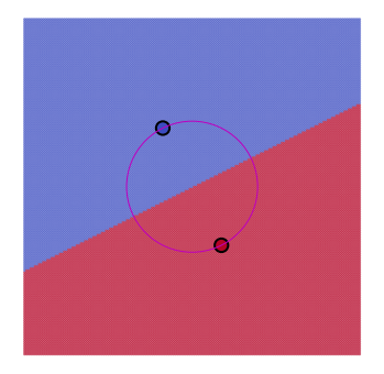
8.7 nex
8.8 Twonex
import numpy as np
import matplotlib.pyplot as plt
from scipy.spatial import Voronoi, voronoi_plot_2d
from sklearn.neighbors import KNeighborsClassifier
Tr = np.array([[-25, 5], [-11, -23], [17, 19], [5, 0], [25, -30]])
Cl = np.array([1, 3, 5, 2, 4])
Nexemplars = Tr.shape[0]
mn = -40
mx = 40
N = 2 * (mx - mn)
Te = np.zeros(((N + 1) ** 2, 2))
for i in range(N + 1):
for j in range(N + 1):
Te[i * (N + 1) + j, 0] = mn + j * (mx - mn) / N
Te[i * (N + 1) + j, 1] = mn + i * (mx - mn) / N
def knn_voronoi_plot(k, Te, Tr, Cl, title):
knn = KNeighborsClassifier(n_neighbors=k)
knn.fit(Tr, Cl)
Lb = knn.predict(Te)
vor = Voronoi(Tr)
fig, ax = plt.subplots()
ax.set_xlim(mn, mx)
ax.set_ylim(mn, mx)
ax.set_aspect('equal')
ax.axis('off')
voronoi_plot_2d(vor, ax=ax, show_vertices=False, line_colors='m', line_width=1)
scatter = ax.scatter(Te[:, 0], Te[:, 1], c=Lb, s=3, cmap=plt.cm.get_cmap('tab10'))
ax.scatter(Tr[:, 0], Tr[:, 1], c=Cl, s=150, marker='o', edgecolor='k', linewidth=2)
ax.set_title(title)
plt.show()
knn_voronoi_plot(1, Te, Tr, Cl, "1-NN with Voronoi Tessellation")
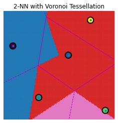
knn_voronoi_plot(2, Te, Tr, Cl, "2-NN with Voronoi Tessellation")
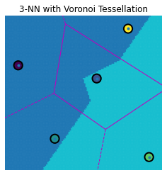
knn_voronoi_plot(3, Te, Tr, Cl, "3-NN with Voronoi Tessellation")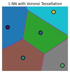
Kmeans-sub
Kmeans
8.9 Knn prob
Knn probdist
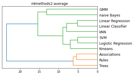
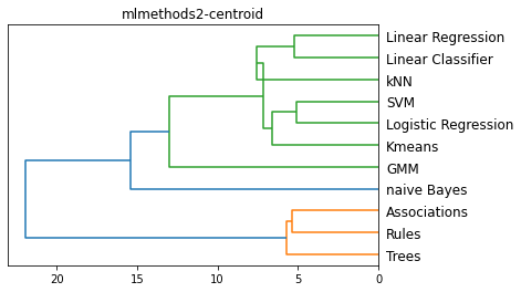
8.12 ML Methoids 2
import numpy as np
import matplotlib.pyplot as plt
from scipy.cluster.hierarchy import linkage, dendrogram
from sklearn.cluster import KMeans
filename = 'mlmethods2'
Names = ['Trees', 'Rules', 'naive Bayes', 'kNN', 'Linear Classifier', 'Linear Regression', 'Logistic Regression', 'SVM', 'Kmeans', 'GMM', 'Associations']
Features = ['geom', 'stat', 'rule', 'split', 'grad', 'symb', 'real', 'sup', 'unsup', 'multi']
M = np.array([
[1, 0, 3, 3, 0, 3, 2, 3, 2, 3],
[0, 0, 3, 3, 1, 3, 2, 3, 0, 2],
[1, 3, 1, 3, 1, 3, 1, 3, 0, 3],
[3, 1, 0, 2, 2, 1, 3, 3, 0, 3],
[3, 0, 0, 0, 3, 1, 3, 3, 0, 0],
[3, 1, 0, 0, 3, 0, 3, 3, 0, 1],
[3, 2, 0, 0, 3, 1, 3, 3, 0, 0],
[2, 2, 0, 0, 3, 2, 3, 3, 0, 0],
[3, 2, 0, 1, 2, 1, 3, 0, 3, 1],
[1, 3, 0, 0, 3, 1, 3, 0, 3, 1],
[0, 0, 3, 3, 0, 3, 1, 0, 3, 1]
])
w1 = 5
w2 = 3
w3 = 1
W = np.array([w1, w1, w1, w2, w2, w3, w3, w3, w3, w3])
D = M * W
methods = ['single', 'complete', 'average', 'centroid']
for m in methods:
plt.figure()
method = m
L = linkage(D, method)
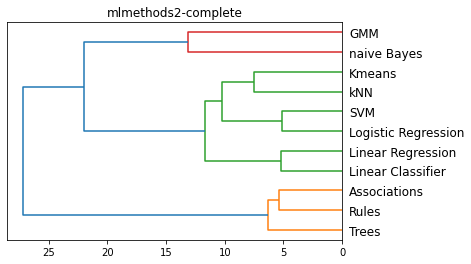
dendrogram(L, color_threshold='default', orientation='left', labels=Names)
plt.title(f'{filename}-{method}')
plt.show()
for k in range(2, 6):
kmeans = KMeans(n_clusters=k, n_init=5, random_state=0)
idx = kmeans.fit_predict(D)
sumd = np.sum(kmeans.inertia_)
print(f'k = {k}, Sum of squared distances (inertia): {sumd}')
for i in range(k):
print(f"Cluster {i + 1}:")
print(np.array(Names)[idx == i]) 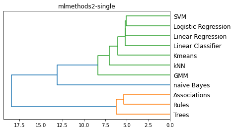
k = 2, Sum of squared distances (inertia): 560.625
Cluster 1:
['naive Bayes' 'kNN' 'Linear Classifier' 'Linear Regression'
 'Logistic Regression' 'SVM' 'Kmeans' 'GMM']
Cluster 2:
['Trees' 'Rules' 'Associations']
k = 3, Sum of squared distances (inertia): 293.5
Cluster 1:
['kNN' 'Linear Classifier' 'Linear Regression' 'Logistic Regression' 'SVM'
 'Kmeans']
Cluster 2:
['Trees' 'Rules' 'Associations']
Cluster 3:
['naive Bayes' 'GMM']
k = 4, Sum of squared distances (inertia): 207.5
Cluster 1:
['naive Bayes']
Cluster 2:
['kNN' 'Linear Classifier' 'Linear Regression' 'Logistic Regression' 'SVM'
 'Kmeans']
Cluster 3:
['GMM']
Cluster 4:
['Trees' 'Rules' 'Associations']
k = 5, Sum of squared distances (inertia): 130.0
Cluster 1:
['GMM']
Cluster 2:
['Trees' 'Rules' 'Associations']
Cluster 3:
['Logistic Regression' 'SVM' 'Kmeans']
Cluster 4:
['kNN' 'Linear Classifier' 'Linear Regression']
Cluster 5:
['naive Bayes']
8.13 ML Kmeans 3
import numpy as np
import matplotlib.pyplot as plt
from sklearn.cluster import KMeans
from sklearn.mixture import GaussianMixture
from sklearn.metrics import silhouette_samples, silhouette_score
from scipy.stats import multivariate_normal
filename = 'mlkmeans3'
sigma = np.array([[1, 0], [0, 1]]) / 10
N = 100
left = np.random.multivariate_normal([1, 0], sigma, N)
right = np.random.multivariate_normal([-1, 0], sigma, N)
data1 = np.vstack((left, right))
data2 = np.tile(np.array([1, 5]), (2 * N, 1)) * data1
k = 2
kmeans1 = KMeans(n_clusters=k, n_init=10, random_state=0).fit(data1)
labels1 = kmeans1.labels_
means1 = kmeans1.cluster_centers_
plt.figure(1)
plt.axis('square')
plt.scatter(data1[:, 0], data1[:, 1], c=labels1, cmap='viridis')
plt.scatter(means1[:, 0], means1[:, 1], c='black', marker='x', s=100)
plt.title(f'{filename}-left')
plt.show()
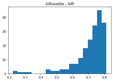
plt.figure(2)
silhouette_vals1 = silhouette_samples(data1, labels1, metric='euclidean')
plt.hist(silhouette_vals1, bins=20)
plt.title('Silhouette - left')
plt.show()
kmeans2 = KMeans(n_clusters=k, n_init=10, random_state=0).fit(data2)
labels2 = kmeans2.labels_
means2 = kmeans2.cluster_centers_
plt.figure(3)
plt.axis('square')
plt.scatter(data2[:, 0], data2[:, 1], c=labels2, cmap='viridis')
plt.scatter(means2[:, 0], means2[:, 1], c='black', marker='x', s=100)
plt.title(f'{filename}-right')
plt.show()
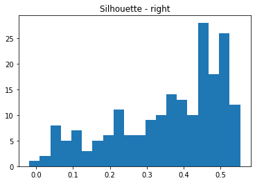
plt.figure(4)
silhouette_vals2 = silhouette_samples(data2, labels2, metric='euclidean')
plt.hist(silhouette_vals2, bins=20)
plt.title('Silhouette - right')
plt.show()
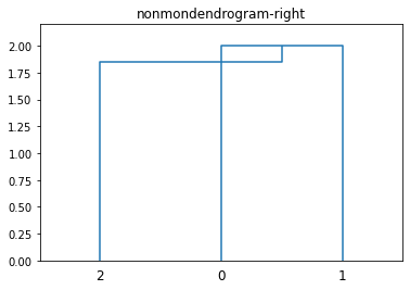
8.17 Nonmon Dendogram
import numpy as np
import matplotlib.pyplot as plt
from scipy.spatial.distance import pdist
from scipy.cluster.hierarchy import linkage, dendrogram
filename = 'nonmondendrogram'
x = 2
d = 0.1
y = np.sqrt((3/4) * x**2 + d * (2 * x + d))
D = np.array([[0, 0], [x, 0], [x / 2, y]]) + 1
methods = ['centroid']
for m in methods:
plt.figure(2)
method = m
L = linkage(D, method)
PD = pdist(D)
dendrogram(L, color_threshold='default')
plt.ylim([0, 2.2])
plt.title(f'{filename}-right')
plt.show()
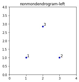
plt.figure(3)
plt.scatter(D[:, 0], D[:, 1], s=20, c='blue', label='Points', marker='o')
plt.axis([0, 4, 0, 4])
plt.gca().set_box_aspect(1)
plt.title(f'{filename}-left')
for i in range(len(D)):
plt.text(D[i, 0] + 0.05, D[i, 1] + 0.05, str(i + 1), fontsize=12)
plt.show()
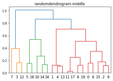
8.18 Random Dendogram
import numpy as np
import matplotlib.pyplot as plt
from scipy.spatial.distance import pdist
from scipy.cluster.hierarchy import linkage, dendrogram, cophenet
from scipy.stats import spearmanr
from sklearn.cluster import AgglomerativeClustering
from sklearn.metrics import silhouette_samples
filename = 'randomdendrogram'
D = np.random.rand(20, 2)
methods = ['complete']
f = 1 Medoids
r, _ = spearmanr(PD, d)
print(f'Spearman correlation for {method}: {r}')
dendrogram(L, color_threshold='default')
plt.title(f'{filename}-middle')
plt.show()
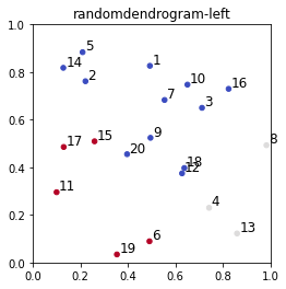
plt.figure(f)
f += 1
clustering = AgglomerativeClustering(n_clusters=3, linkage=method)
T = clustering.fit_predict(D)
plt.scatter(D[:, 0], D[:, 1], s=20, c=T, cmap='coolwarm', marker='o')
d = 0.01
for i in range(D.shape[0]):
plt.text(D[i, 0] + d, D[i, 1] + d, str(i + 1), fontsize=12)
plt.title(f'{filename}-left')
plt.axis([0, 1, 0, 1])
plt.gca().set_box_aspect(1)
plt.show()
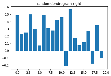
plt.figure(f)
f += 1
silhouette_vals = silhouette_samples(D, T, metric='euclidean')
plt.bar(range(D.shape[0]), silhouette_vals)
plt.title(f'{filename}-right')
plt.show()Spearman correlation for complete: 0.5691352429297899
Silhouette
Twonex
import numpy as np
import matplotlib.pyplot as plt
from scipy.spatial import Voronoi, voronoi_plot_2d
from sklearn.neighbors import KNeighborsClassifier

Tr = np.array([[-25, 5], [-11, -23], [17, 19], [5, 0], [25, -30]])
Cl = np.array([1, 3, 5, 2, 4])

Nexemplars = Tr.shape[0]

mn = -40
mx = 40
N = 2 * (mx - mn)

Te = np.zeros(((N + 1) ** 2, 2))
for i in range(N + 1):
    for j in range(N + 1):
        Te[i * (N + 1) + j, 0] = mn + j * (mx - mn) / N
        Te[i * (N + 1) + j, 1] = mn + i * (mx - mn) / N

def knn_voronoi_plot(k, Te, Tr, Cl, title):
    knn = KNeighborsClassifier(n_neighbors=k)
    knn.fit(Tr, Cl)
    Lb = knn.predict(Te)

    vor = Voronoi(Tr)

    fig, ax = plt.subplots()
    ax.set_xlim(mn, mx)
    ax.set_ylim(mn, mx)
    ax.set_aspect('equal')
    ax.axis('off')

    voronoi_plot_2d(vor, ax=ax, show_vertices=False, line_colors='m', line_width=1)

    scatter = ax.scatter(Te[:, 0], Te[:, 1], c=Lb, s=3, cmap=plt.cm.get_cmap('tab10'))

    ax.scatter(Tr[:, 0], Tr[:, 1], c=Cl, s=150, marker='o', edgecolor='k', linewidth=2)

    ax.set_title(title)
    plt.show()

knn_voronoi_plot(1, Te, Tr, Cl, "1-NN with Voronoi Tessellation")

knn_voronoi_plot(2, Te, Tr, Cl, "2-NN with Voronoi Tessellation")

knn_voronoi_plot(3, Te, Tr, Cl, "3-NN with Voronoi Tessellation")